
Consider a stream of data that we receive, call them  where
where  is the
  element in the stream. Note that we receive every at the time step and that is then no more in our access once we move on to the next time step. Furthermore, we don’t even know the value of
  . How can we possibly uniformly sample an element from this stream? When I first thought about this, I was completely stuck; I couldn’t fathom any such procedure; to me, it just felt wrong that we needed to gain a uniform sample over samples without even knowing !
However, as the title implies, one method to accomplish this is called Reservoir Sampling. I’ll first introduce the mechanics directly, and don’t be discouraged if it doesn’t make sense since it can be quite non-intuitive at first. Before we delve into the mathematics, I recommend you take a look at this post, especially the basics of probability theory.
Development of the Theory
First, we let our stream be  and we start by seeing
  and continue all the way to
  . Now consider the random variables
  defined by

In other words, we keep a reservoir sample and switch it to the current element we are reading with probability inverse to the current timestep, and the variables simply are the state of the reservoir at different timesteps. We claim that
![\begin{align*} \Pr[X_n = x_i] = \frac{1}{n}, \end{align*}](https://balaramdb.com/wp-content/ql-cache/quicklatex.com-f2ce5be7fe8c43c8317586d852806dec_l3.png "Rendered by QuickLaTeX.com")
for all  , i.e.
  is a uniformly distributed random variable from the sample space of all the stream elements. And in fact, we define as our sample from the stream.
Now what confused me the most was that the probability that  (fixing
  ) is
) is  is
is  , but then somehow we concluded the probability that remains as is
  . Seemingly confusing, right? We may select at the
  timestep; however, we forget that we still need to not select the rest of the elements in order for to remain . That part about not selecting other elements weighs into proving that is uniformly distributed, and now we will see this in motion formally. I will provide a rigorous proof first, and then a more intuitive argument afterward.
Claim: Defining and as we have, we claim
![\begin{align*} \Pr[X_n = x_i] = \frac{1}{n}. \end{align*}](https://balaramdb.com/wp-content/ql-cache/quicklatex.com-2a06926faf570ead03419137ec630cc8_l3.png "Rendered by QuickLaTeX.com")
Proof: We prove the claim by induction on . First consider the case of  where then we choose the first and only element of the stream with full probability, so obviously our selection is uniform.
Now consider some arbitrary  , and assume the claim for the stream . Now add an element
  to the stream, so our stream is
  now. Now by definition
  with probability
  , so for all
  :
:
![\begin{align*} \Pr[X_{n + 1} = x_j] &= \Pr[(X_{n + 1} = X_n) \cap (X_n = x_j)] \\ &= \Pr[X_{n + 1} = X_n] \Pr[X_n = x_j \mid X_{n + 1} = X_n] \\ &= \Pr[X_{n + 1} = X_n] \Pr[X_n = x_j] \\ &= \lp1 - \frac{1}{n + 1}\rp \lp \frac{1}{n} \rp \\ &=\frac{n}{n + 1} \cdot \frac{1}{n} \\ &= \frac{1}{n + 1} \end{align*}](https://balaramdb.com/wp-content/ql-cache/quicklatex.com-45a3ea54b28cdfe9f9d241d415db08c3_l3.png "Rendered by QuickLaTeX.com")
as required. The second line is by Conditional Equivalence (details can be found here), the third by the independence of the reservoir’s state at a previous timestep, and the fourth derived from the inductive hypothesis. Furthermore, by definition we know ![\Pr[X_{n + 1} = x_{n + 1}] = \frac{1}{n + 1}](https://balaramdb.com/wp-content/ql-cache/quicklatex.com-d1cc0158a10fa5971d8db26909cded9c_l3.png "Rendered by QuickLaTeX.com") . Thus we have shown for all
. Thus we have shown for all  :
:
![\begin{align*} \Pr[X_{n + 1} = x_i] = \frac{1}{n + 1}, \end{align*}](https://balaramdb.com/wp-content/ql-cache/quicklatex.com-b422cfd21959112c165128cfd35e1fc5_l3.png "Rendered by QuickLaTeX.com")
i.e.  is an uniform sample from the stream as claimed; thus proving the correctness of Reservoir Sampling.
A more intuitive approach, although less rigorous, is by writing
![\begin{align*} \Pr[X_n = x_j] = \Pr[X_j = x_j] \cdot \prod_{i = j + 1}^n \Pr[X_i = X_{i - 1}] \end{align*}](https://balaramdb.com/wp-content/ql-cache/quicklatex.com-9b752a6ba813c3ed2148253d428d84a8_l3.png "Rendered by QuickLaTeX.com")
which is essentially the probability we select and then never select any other element of the stream. We can simplify:
![\begin{align*} \Pr[X_n = x_j] &= \frac{1}{j} \cdot \prod_{i = j + 1}^n \lp 1 - \frac{1}{i} \rp \\ &= \frac{1}{j} \cdot \prod_{i = j + 1}^n \lp \frac{i - 1}{i} \rp \\ &= \lp \frac{1}{j} \rp \lp \frac{j}{j + 1} \rp \cdots \lp \frac{n - 1}{n} \rp \\ &= \frac{1}{n} \end{align*}](https://balaramdb.com/wp-content/ql-cache/quicklatex.com-c6483580a9093bf06454ab467b4bb55f_l3.png "Rendered by QuickLaTeX.com")
as required, so we have shown that is uniform. This isn’t rigorous since we haven’t had a chance to discuss the relations between the random variables in order to get that initial product, and we never need to delve into that with our proof by induction.
Verifying Reservoir Sampling
Now that we have understood the theory of Reservoir Sampling, let’s take a look at it in full motion. The following is the Python code for the Reservoir Sampling Algorithm.
def get_reservoir_sample(stream):
  n = len(stream)
  X = 0 # our sample
  for i in range(n):
    if rand.random() < 1/(i + 1):
      X = stream[i]
  return X
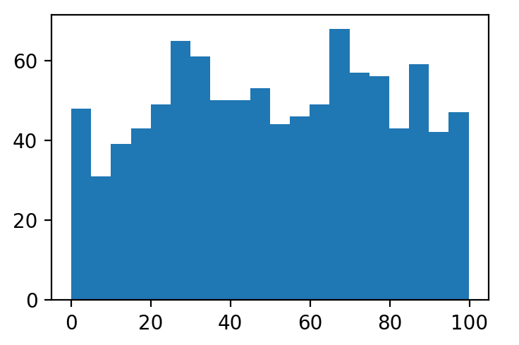
Now we generate a stream of 1,000 elements whose distribution is depicted in the following histogram.
Now after sampling 10,000 elements by the Reservoir Sampling, we arrive at the following distribution of samples.
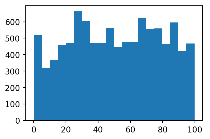
Notice that the distributions are almost identical which verifies the uniformity of the Reservoir Sampling in practice.
I encourage you to try this for yourself and witness the power of Reservoir Sampling.
Practical Use of Reservoir Sampling
Common in most Streaming Algorithms, we tend to assume our stream to be extremely large, so storing the contents of the stream in memory is simply not viable. For example, consider a stream of posts from all CS blogs; obviously, storing each one in memory is a waste of space, but with Reservoir Sampling we can sample one post uniformly with  space compared to
  if we decided to keep all the posts.
Furthermore, if we need  independent samples from a stream, we can Reservoir Sample simultaneously and independently, so we can get our samples with only one pass through the stream. In practice, this method tends to be the preferred method of sampling as often we need more than just one sample.
Also, there are more applications of this principle of keeping a reservoir (the samples) and replacing it with new stream elements as time passes, so look out for posts on this topic of streaming algorithms.
Recent Comments