Introduction to Probability Distributions

There are many methods of introducing structure to random variables in Probability Theory, and traditionally we call this structure a property, and one such property is its distribution. Phrases like “coming from this distribution” or “they distribute as such” or “these variables make this distribution” all refer to this property. In this post, we will go into the most common distribution and introduce basic facts for each one.

This post is part of a multi-post series going over such distributions, and for more detailed analysis and writing, look out for the next few posts.

Many of the explanations and facts are referenced from Probability and Computing by Mitzenmacher and Upfal and William Feller’s classic An Introduction to Probability Theory.

Probability Theory Basics

Before we begin, let’s start from the very basics. Let’s define our sample space $\Omega$ which is the set of all possible samples. Now an event $A$ is a subset of the sample space, i.e. it is a collection of samples. Further, we can define any event $A$ in the power set of $\Omega$ , denoted by $\sP(\Omega)$ , which is the set of all subsets of $\Omega$ . Intuitively, an event entails a set of samples that represent when that event happens. For example, in the sample space of weather forecasts of every day in the year, we have an event $R$ when it rains, so $R$ is the set of all days in the year when it rained.

Having defined the sample space and event, let’s define probability. Intuitively, it signifies how likely an event is to occur, and mathematically we define it as follows.

Definition 1: A probability function is a function $\Pr: \sP(\Omega) \to \R$ where

for all events $A$ , we have $0 \le \Pr[A] \le 1$ ;
we have $\Pr[\Omega] = 1$ ; and
for any countably infinite mutually disjoint collection of events $A_1, A_2, \ldots$ , we have

$\begin{align*}\Pr\lp \bigcup_{i \ge 1} A_i \rp = \sum_{i \ge 1} \Pr[A_i].\end{align*}$

Now we’ll define the random variable, which will be playing a key role in all our probabilistic analyses. The following definition is extremely abstract primarily because we want it to have flexible structure for future use.

Definition 2: A random variable $X$ over $\Omega$ is a real-valued function $X: \Omega \to \R$ .

Notice that we can let $A$ be the event where some random variable $X = x$ where $x \in \R$ , and then we see that $\Pr[A] = \Pr[X = x]$ and to understand this probability, we require some knowledge of the randomness. That is described by the distribution which essentially defines the probability function for a random variable. We will explore these facts soon, but before we get there let’s continue with our introduction to the basics of probability theory.

Now we will define expectation, and its mathematical definition is just like its literal one. We denote by $\EX[X]$ , and by definition it is

$\begin{align*}\EX[X] = \sum_x x\Pr[X = x],\end{align*}$

and in most of our uses of expectation, the sum converges to a real number. Essentially, $\EX[X]$ is the expected value of $X$ .

We must introduce the two key facts; note the first one is more of a definition, and the second has a brief proof.

Fact 1 (Conditional Equivalence): For two events $A_1$ and $A_2$ , we have

$\Pr[A_1 \cap A_2] = \Pr[A_1] \Pr[A_2 | A_1].$

Fact 2 (Linearity of Expectation): For two random variables $X$ and $Y$ ,

$\EX[X + Y] = \EX[X] + \EX[Y].$

Proof: By definition we have where $z = x + y$ :

$\begin{align*} \EX[X + Y] &= \sum_z z \Pr[X + Y = z] \\&= \sum_{x, y} (x + y) \Pr[X = x \text{ and } Y = y] \\&= \sum_{x, y} x \Pr[X = x \text{ and } Y = y] \\&\quad\quad+ \sum_{x, y} y \Pr[Y = y\text{ and } X = x] \\&= \sum_{x, y} x \Pr[X = x] \Pr[Y = y \mid X = x] \\&\quad\quad+ \sum_{x, y} y \Pr[Y = y] \Pr[X = x \mid Y = y] \\&= \sum_x x \Pr[X = x] \sum_y \Pr[Y = y \mid X = x] \\&\quad\quad+ \sum_y y \Pr[Y = y] \sum_x \Pr[X = x \mid Y = y] \\&= \sum_x x \Pr[X = x] (1) + \sum_y y \Pr[Y = y] (1) \\&= \EX[X] + \EX[Y], \end{align*}$

where the fourth line comes from Conditional Equivalence, the sixth from the fact that $\sum_s \Pr[S = s \mid T = t] = 1$ for fixed $t$ and random variables $S$ and $T$ , and the last line by the definition of expectation. Thus we have proved the linearity of expectations. $\quad \blacksquare$

Note that the form $\Pr[B | C]$ for events $B$ and $C$ is the probability that $B$ occurs conditioned on $C$ occurring, and we call this conditional probability and it is defined by Conditional Equivalence.

Lastly, let’s introduce the notion of variance. We denote it by $\var[X]$ and define it as

$\begin{align*}\var[X] = \EX[(X - \EX[X])^2].\end{align*}$

And the important expression to note is $X - \EX[X]$ which is essentially the deviance of the random variable from its expectation, and then we square it to weed out the role of the sign. Thus we define the variance as the expected deviance squared.

Further, by Linearity of Expectation, we get

$\begin{align*}\var[X] &= \EX[(X - \EX[X])^2] \\&= \EX[X^2 - 2X\EX[X] + (\EX[X])^2] \\&= \EX[X^2] - \EX[2X\EX[X]] + \EX[(\EX[X])^2] \\&= \EX[X^2] - 2\EX[X]\cdot\EX[X] + (\EX[X])^2 \\&= \EX[X^2] - (\EX[X])^2.\end{align*}$

Note that we used the fact that the expectation of the expectation is simply the expectation, e.g. $\EX[\EX[X]] = \EX[X]$ . Thus we derived another definition of variance as

$\var[X] = \EX[X^2] - (\EX[X])^2.$

Now another form that most are usually familiar with is the standard deviation which, denoted by the $\simga$ , is defined as

$\sigma[X] = \sqrt{\var[X]}.$

We will frequently use these terms when we go into concentration inequalities, but they are introduced here to enhance our introduction to probability distributions.

Uniform Distribution

We are familiar with the coin toss or the dice roll, and what’s common with most of these experiments is that there is an equal chance for any option: there is a $\frac{1}{2}$ chance that a coin flips as head or tail and there is a $\frac{1}{6}$ chance that a dice rolls as a $1$ , $2$ , $3$ , $4$ , $5$ , or $6$ . This is what we call the uniform distribution, where all options have equal probability.

Definition 3: A random variable $X$ from the uniform distribution with parameter $n$ is defined by the probability distribution for all $x = 1, \ldots, n$ , we have

$\Pr[X = x] = \frac{1}{n}.$

The parameter $n$ signifies the number of options we have in our distribution, and thus the probability that $X$ is any one of the options is $\frac{1}{n}$ .

A generalization of the uniform distribution is called the categorical distribution or the multinomial distribution which will be discussed in an upcoming post.

Normal Distribution and Bell Curve

We have all heard of the “curve,” usually in the setting of grading or assorting data in the real world. Please note this curve is not the same as the curve of the COVID-19 pandemic (in full swing while this post was written); that curve refers to the derivative of the logistic curve. The curve I am referring is the famous Bell Curve which receives its name by how it is shaped.

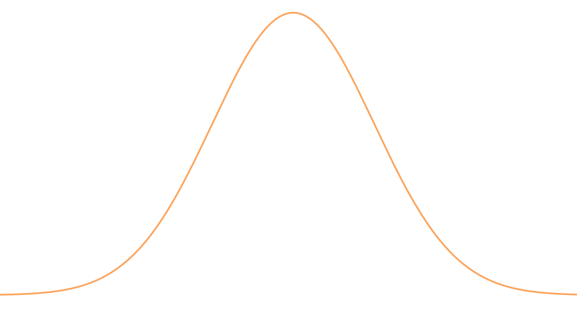
The above figure is a generic Bell Curve, and notice that it is symmetric and its peak is where its mean stands. Further, notice that the “width” or “stretch” of the curve would say something about deviance as well.

This curve is the Probability Density Function (PDF) of the Normal distribution. Let’s unpack that a little. Remember how we defined probability as a function; the PDF is merely another way of referring to that function. This curve is essentially a definition of the function, and that definition is what we call the Normal distribution. It’s called the normal distribution since many observations of nature fit into this curve. For example, the heights of males fit this curve, or even how well students score on a test; the examples are endless, and this is why theorists tend to spend a lot of time understanding this distribution to gain a better sense of our world in general.

Along with the physical examples, the features of this distribution are quite convenient in analysis which we will explore deeply in an upcoming post, going over the mechanics of this key distribution.

On a final note, this distribution is also called the Gaussian distribution, and the Bell Curve the Gaussian Curve, and this notation is more scientific and more commonly used in research.

Bernoulli Random Variables and Binomial Distribution

Finally, we can begin getting to the real content of this blog post. In all our discussion on these distributions we plan to give basic intuition and short examples, and for more formal mathematics and elaborate examples look out for more blog posts focused on each distribution.

First, let’s talk about one of the most common random variables. A lot of events can be converted to decision events, i.e. either the event occurs or doesn’t. For example, let’s again take the example of the weather, and narrow it down to either it rained or didn’t. We can let some variable $X$ indicate whether it rained or not by

$\begin{align*}X = \begin{cases} 0 & \text{ if it didn't rain} \\ 1 & \text{ if it rained} \end{cases}\end{align*}$

In this case, we call this variable $X$ a Bernoulli because it is either 0 or 1. We can also call $X$ an indicator because it indicates some implied event. These variables are the most commonly used in randomized algorithms.

A generalization of the Bernoulli is the Binomial random variable which comes from the Binomial distribution. An example of the distribution is shown below.

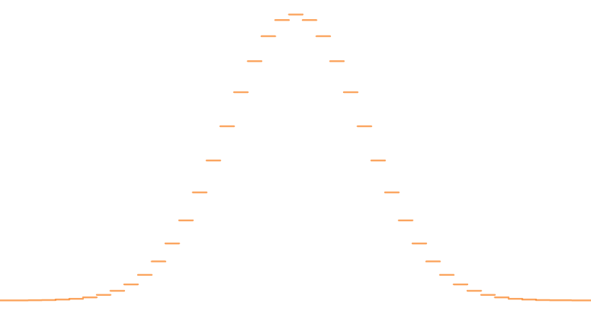
As we can see, this is a discrete distribution, and the full specifics of this will be discussed in another post. There are continuous approximations of this variable such as the Beta distribution, but those are reserved for another time.

Geometric Distribution

Now we are venturing into the range of the less commonly discussed distributions. What if we had a random variable that was memory invariant, i.e. the distribution of the random variable remains the same under all conditions? This is precisely what the Geometric random variable offers. To clarify, for the Geometric random variable $X$ , we have

$\begin{align*} \Pr[X = n + k \mid X > k] = \Pr[X = k] \end{align*}$

for all $n$ and $k$ . Isn’t that pretty sweet?

To graphically depict this phenomenon, the following is an example of the Geometric distribution.

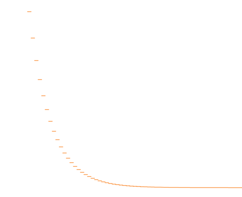
Since the area under the PDF must be one, keeping this memoryless property is extremely special. It essentially says that by starting from any point on the x-axis, the curve will look the same if scaled according to the probability at that point. This special property is a gift of the exponential.

The continuous version of the Geometric distribution is called the Exponential Distribution, and its definition is similar to the former. Look out for more posts regarding this distribution and the Coupon Collector Problem which is a famous problem applying Geometric random variables in its analysis.

Poisson Distribution

We won’t be able to explore the applications of the Poisson distribution, but we will try to give a brief introduction to a setting that uses Poissons, as they are called. The following image is an example of the Poisson distribution.

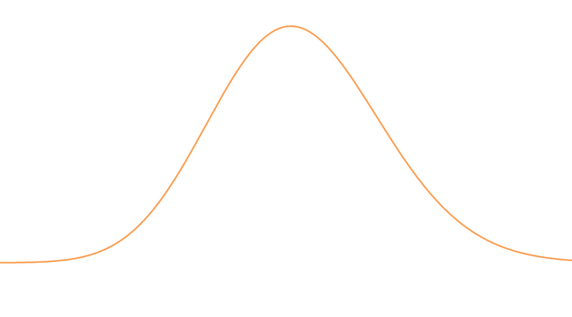
It may difficult to notice, but its not truly symmetric, yet its shape mimics the Binomial distribution and the Normal distribution, and we will see that we use this distribution to approximate other distributions to gain more freedom with independence.

Furthermore, this distribution is highly used in the Balls and Bins setting: where we have $n$ bins and randomly assort $m$ balls to the bins. In order to solve problems in this setting like the Max Load problem — to find the maximum number of balls in a bin — we can use Poisson Approximation. Note that hash function analysis is essentially a case of Balls and Bins, and this marks one of the prominent uses of this setting and Poissons.

Looking Forward

I plan to eventually go into the definitions of these distributions, the expectation, and variance that come with the distributions, and some elaborate examples to cement the intuition and theory. Note that, the reason I am beginning with such an introduction to Probability Theory is that it will form the basis of a lot of Randomized Algorithms, and I plan to go into those in the future. One example of such a field would be Property Testing, where we try to determine whether some given distribution matches some target distribution. Furthermore, simply knowing these distributions can advance mathematical literacy and aide in most future reading, and this post will serve as a brief reference for my future posts.

Thank you for reading through my first official blog post!

Recent Posts

Recent Comments

Subscribe

Categories

Archives

Introduction to Probability Distributions

Probability Theory Basics

Uniform Distribution

Normal Distribution and Bell Curve

Bernoulli Random Variables and Binomial Distribution

Geometric Distribution

Poisson Distribution

Looking Forward

About the Author

Balaram Behera

2 thoughts on “Introduction to Probability Distributions”

Leave a Reply Cancel reply

You may also like these

Key Probabilistic Concentration Bounds

Measure Theoretic Probability Theory

Reservoir Sampling: Uniform Sampling of Streaming Data