Analysis of Randomized QuickSort

The Randomized QuickSort sorting algorithm is a foundational randomized algorithm whose randomized analysis is always imperative to absorb and internalize. In this post, we explore the very simplified approach to its analysis with the use of probabilistic techniques rather than a brute-force expected run-time analysis.

The procedure and intuition behind this algorithm are comprehensively described in a previous post, and the key probabilistic background that will be employed here can also be found in a previous post. Here, we first begin with a discussion addressing the fact that we analyze expected run-time not average-case run-time, and then move on to some empirical results that motivate the discussion of expected run-time analysis (more intuitive motivation can be found in my previous post). Then we will quickly discuss the brute-force method to simply emphasize the goriness of the analysis; then we lastly move on to a simpler and cleaner analysis.

Some facets of this analysis are adapted from Introduction to Algorithms, 3rd Ed., Chapter 7 by Cormen et. al., and also from Prof. C. Seshadhri’s lecture notes from his CSE 290A course at UC Santa Cruz; these notes can be found here, and the lecture recording can be found here.

Expected Run-time vs. Average Run-time

When I first explored QuickSort’s analysis it was labeled by “average run-time”, but an average over what? Is it over all possible input arrays? This notion makes sense for a deterministic algorithm where we want to see the behavior of the algorithm over all input, and we call this the average run-time of the algorithm.

Applying this notion to our problem setting, the average run-time for deterministic QuickSort is then $O(n\log (n))$ since, on average, the last element of the array is a balanced pivot. However, this isn’t very helpful since we have a very real worst-case input of a sorted or reverse sorted array input.

On the other hand, for Randomized QuickSort, given some array $A$ , the expected run-time of Randomized QuickSort is the expected run-time over all possible ways the randomized algorithm could sort the array. This makes sense since we choose our pivot randomly, so there can be different run-times, so we look for the expected run-time. As we will derive further in this blog, this expected run-time is also $O(n \log n))$ .

From above we see that both the expected run-time and average run-time are asymptotically the same (both are $O(n \log n)$ ). This is special to QuickSort since the randomization of choosing the pivot is the only difference between Randomized QuickSort and deterministic QuickSort, and so with randomization of input arrays, the benefit of randomly choosing a pivot is essentially nullified. This, although not formal, can give some intuition as to why both the expected run-time and average run-time are similar. For the formal conclusion, it requires some intensive probability theory and conditional probability, so rather we will explore this in the section to empirically confirm our conclusions here.

Empirical Motivation

Here we wish to explore some empirical results on the number of array comparisons made by both the deterministic and randomized versions of QuickSort. As a disclaimer, the results are quite underwhelming hinted by our discussion regarding the two different metrics for run-time.

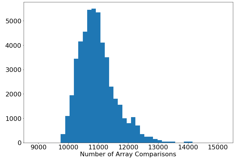
We counted the number of array comparisons (which we will deem as the run-time in our case since it is arguably the most expensive operation in our QuickSort algorithms) made by the regular deterministic QuickSort with a random array input. We did this over 1,000 arrays of size 1,000 (note we ran QuickSort 50 times on the same array to make the magnitude the same as for the next plot to aid in comparing the two), and the distribution of run-time is shown below.

Distribution of Run-time of QuickSort Over Random Array Inputs (Histogram Plot)

Then we do the same for Randomized QuickSort, but this time on the same array we ran the algorithm 50 times as to get a nice idea of the distribution of Randomized QuickSort on randomized input arrays which is shown below.

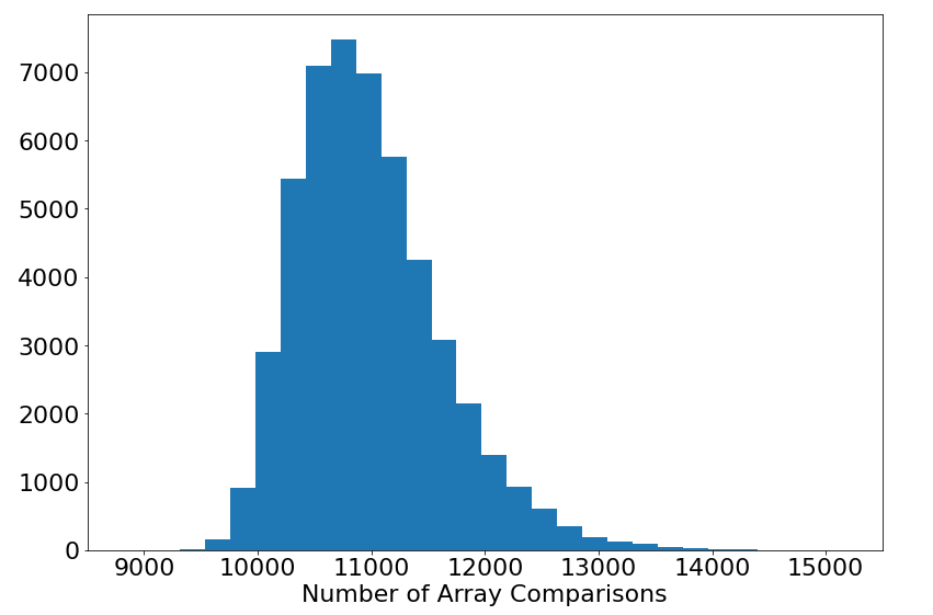
Distribution of Run-time of Randomized QuickSort Over Random Array Inputs (Histogram Plot)

As foreshadowed, the plots are extremely similar in their shape and mean, and in fact, this was expected by our analysis in the last section that the expected running time and average running time would be asymptotically the same.

Then this begs to ask what even is the advantage of Randomized QuickSort? What it guarantees is an expected run-time of $O(n \log n)$ on any given input, and without the randomness, we have a deterministic run-time for a given input which isn’t desirable all the time. This can be seen in the following plot which depicts the run-time distribution for some given instance (over 1,000 samples with an array of length 1,000).

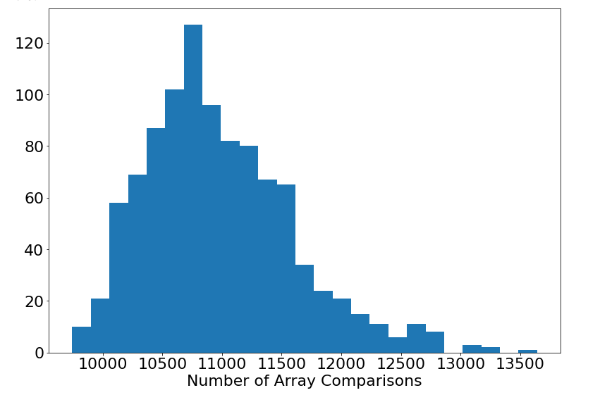
Distribution of Run-time of Randomized QuickSort on a Fixed Random Input Array (Histogram Plot)

The deterministic QuickSort for this array takes 10,457 array comparisons as well which is close to the mean which is expected since we ran this over a random input.

However, let’s look into the most problematic case for QuickSort which is the reverse-sorted array. The deterministic version of QuickSort takes 499,500 array comparisons with is quite mammoth, but Randomized QuickSort’s run-time on the same reverse-sorted array is given by the following distribution over 1,000 samples again.

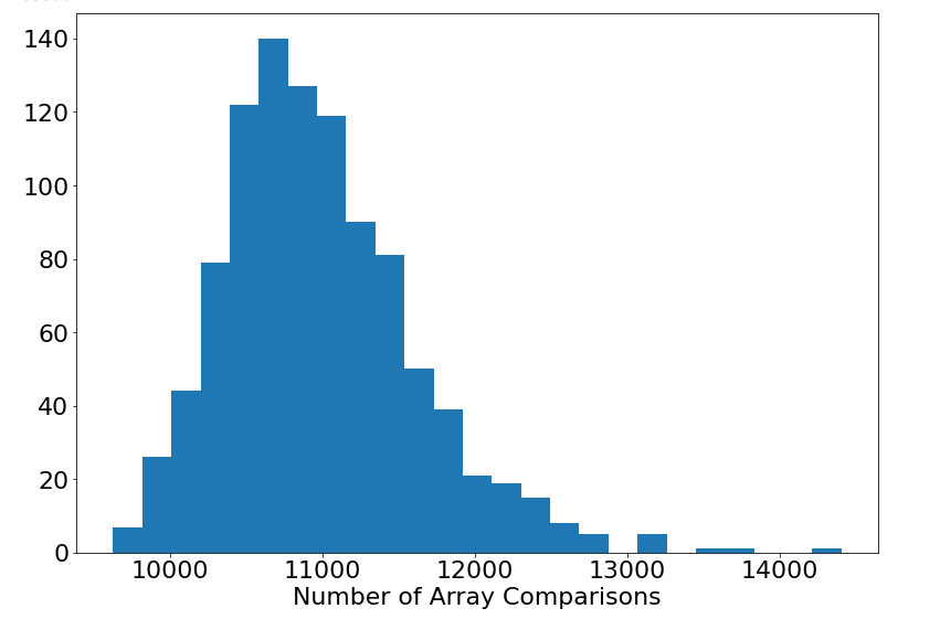
Distribution of Run-time of Randomized QuickSort on a Fixed Reverse-sorted Input Array (Histogram Plot)

The result here is amazing introducing a stark contrast. We never even require more than 15,000 array comparisons to sort the previously problematic reverse-sorted array. This is an extreme example, but it also presents the extreme benefits of randomization and its power of generalizing an algorithm’s utility regardless of the input.

Thus we emphasize the randomized version due to this extra guarantee we have that enhances our algorithm’s general effectiveness and speed. The discussion in this section aimed to provide some empirical motivation in this light.

Brute-Force Analysis

Consider an array $A$ of $n$ elements. Now suppose we have chosen a pivot $p$ from $A$ uniformly at random, and subsequently partitioned the array into sub-arrays $L$ and $R$ where $L$ includes all the elements of $A$ (excluding $p$ ) that are at most $p$ and $R$ includes all elements of $A$ that are greater than $p$ . Let $T(n)$ be the run-time of Randomized QuickSort on array $A$ of $n$ elements. From the preceding post on Randomized QuickSort (found here), we realize that

$\begin{align*} T(n) = T(|L|) + T(|R|) + O(n) \end{align*}$

considering that it takes $O(n)$ time to generate the partitions by comparing every element of $A$ to the chosen pivot $p$ .

To find our expected run-time, we can simply consider that $T(n)$ is a random variable since of course its value is dependent on the randomness of the pivot’s choice, so we want to find $\EX[T(n)]$ , where $\EX[.]$ denotes expectation. So it further follows by the definition of expectation that

$\begin{align*} \EX[T(n)] = \sum_{k = 0}^n \lp \Pr[|R| = k] \rp \lp T(n - k - 1) + T(k) + O(n) \rp \end{align*}$

since we can consider $|R|$ to be a random variable since it depends on the random variable $p$ . Now in order to compute the above expression, we need to understand the distribution of $|R|$ . Observe that for there to be precisely $k$ elements in $A$ that are greater than the uniformly chosen at random pivot, $p$ must be the $(n - k)$ ‘th element of $A^*$ (the sorted version of $A$ ), denoted by $A^*_{n - k}$ , which follows that

$\begin{align*} \Pr[|R| = k] = \Pr[A^*_{n - k} = p] = \frac{1}{n} \end{align*}$

since $p$ is chosen uniformly at random from $A$ . Thus by substituting to an above expression we finally achieve

$\begin{align*} \EX[T(n)] &= \frac{1}{n} \sum_{k = 0}^n \lp T(n - k - 1) + T(k) + O(n) \rp \\ &= O(n) + \frac{1}{n} \sum_{k = 0}^n \lp T(n - k - 1) + T(k) \rp \end{align*}$

and fully computing this expression is a very lengthy process and provides little intuition or satisfaction to understand why the average case performs so well in comparison to the worst-case run-time, so we avoid further computation with this brute-force method.

Preliminaries of a Simpler Analysis

Implicitly, we have been defining run-time considering that the array comparison operation (the action of comparing two elements in an array) is the most expensive operation in the algorithm since we are only moving around elements of the input array in the process of sorting, and that operation occurs only when we make a comparison. Thus, under this assumption (which of course is very well-founded), by simply computing the expected number of array comparisons on some fixed input array, we can realize the expected run-time of Randomized QuickSort.

In regards to notation, let’s continue to suppose that $A^*$ denotes the sorted array of the input array $A$ , and of course, assume that the length of the array $A$ is $n$ .

We define the random variable $X_{i, j}$ to indicate whether $A^*_i$ is compared to $A_j^*$ in the computation of Randomized QuickSort. Note that the comparison between two elements in the array can happen at most once since one must be the pivot and will be omitted from both $L$ and $R$ .

Considering the most expensive operation being the comparison of two array elements, computing the number of array comparisons is equivalent to the run-time. Thus $\EX\left[ \sum_{i < j} X_{i, j} \right]$ is the expected the run-time of Randomized QuickSort. By the Linearity of Expectation, we get

$\begin{align*} \EX\left[ \sum_{i < j} X_{i, j} \right] = \sum_{i < j} \EX[X_{i, j}]. \end{align*}$

Thus, it should be sufficient to compute $\EX[X_{i, j}]$ for any $i < j$ .

The Probabilistic Analysis

In our following computation, we cleverly utilize the pivot’s ability to separate an array into $L$ and $R$ .

Lemma: For any $i < j$ , we have $\EX[X_{i, j}] = \frac{2}{j - i + 1}$ .

Proof: We prove this by induction on the size of the array, denoted by $n$ . In the base case of $n = 2$ , we only have s $i = 1$ and $j = 2$ , thus $\frac{2}{j - i + 1} = 1$ . This is consistent because Randomized QuickSort will compare the only two elements in the array in order to sort them, and thus $\EX[X_{i, j}] = 1$ .

Choose arbitrary $n > 2$ , and assume the inductive hypothesis for all arrays of size less than $n$ . Further, since $X_{i, j}$ is in indicator (i.e. it is equal to 1 if true and 0 if false), we can write

$\begin{align*} \EX[X_{i, j}] = \Pr[X_{i, j} = 1]. \end{align*}$

Let the first pivot of Randomized QuickSort on the array $A$ be the element $p$ , and let $L$ and $R$ be the corresponding “left” and “right” side of $A$ after pivoting. Further note that since $i < j$ and since $A^*$ is sorted, we get $A^*_i < A^*_j$ . Essentially, we can consider three cases for $A^*$ which we informally depict below:

$\begin{align*} A^* &= [\cdots A^*_i \cdots A^*_j \cdots p \cdots] \\ A^* &= [\cdots p \cdots A^*_i \cdots A^*_j \cdots] \\ A^* &= [\cdots A^*_i \cdots p \cdots A^*_j \cdots] \end{align*}$

Therefore, by the Law of Total Probability, we can alternatively write

$\begin{align*} \Pr[X_{i, j} = 1] &= \Pr[X_{i, j} = 1 \mid A^*_j < p] \, \Pr[A^*_j < p] \\ &\quad + \Pr[X_{i, j} = 1 \mid A^*_i > p] \, \Pr[A^*_i > p] \\ &\quad + \Pr[X_{i, j} = 1 \mid A^*_i \le p \le A^*_j] \, \Pr[A^*_i \le p \le A^*_j]. \end{align*}$

If $A^*_j < p$ , then that means both $A^*_i$ and $A^*_j$ are in $L$ , and so by induction on $L$ , we have

$\begin{align*} \Pr[X_{i, j} = 1 \mid A^*_j < p] = \frac{2}{j - i + 1}. \end{align*}$

Similarly, if $A^*_i > p$ , then both $A^*_i$ and $A^*_j$ are in $R$ , and so

$\begin{align*} \Pr[X_{i, j} = 1 \mid A^*_i > p] = \frac{2}{j - i + 1}. \end{align*}$

In the case where $A^*_i \le p \le A^*_j$ , the only way $A^*_i$ and $A^*_j$ are being compared to each other are if either one is the pivot (because otherwise, $A^*_i$ would be in $L$ and $A^*_j$ would be in $R$ and they would never be compared in the Randomized QuickSort algorithm). Thus, the probability of either being the pivot is $\frac{2}{j - i + 1}$ by counting, so

$\begin{align*} \Pr[X_{i, j} = 1 \mid A^*_i < p < A^*_j] = \frac{2}{j - i + 1}. \end{align*}$

Hence, by substition,

$\begin{align*} \Pr[X_{i, j} = 1] &= \frac{2}{j - i + 1} \left( \Pr[A^*_j < p] + \Pr[A^*_i > p] + \Pr[A^*_i \le p \le A^*_j] \right) \\&= \frac{2}{j - i + 1}. \end{align*}$

as claimed. $\blacksquare$

Thus bringing it all together, we have the central theorem below.

Theorem: The expected run-time of Randomized QuickSort is $O(n \log n)$ ; in particular,

$\begin{align*} \sum_{i < j} \EX[X_{i, j}] \le 2nH_n \end{align*}$

where $H_n$ is the Harmonic Series.

Proof: Note that we consider the number of comparisons as equivalent to the run-time of Randomized QuickSort, and we wish to compute the expected run-time, i.e. to compute $\sum_{i < j} \EX[X_{i, j}]$ . We can expand as follows by the previous lemma:

$\begin{align*}\sum_{i < j} \EX[X_{i, j}] &= \sum_{i < j} \frac{2}{j - i + 1} \\&= \sum_{i = 1}^{n - 1} \sum_{j = i + 1}^{n} \frac{2}{j - i + 1} \\&= \sum_{i = 1}^{n - 1} \sum_{k = 1}^{n - i} \frac{2}{k + 1} \\&= \sum_{i = 1}^{n - 1} 2(H_{n - i} - 1) \\&\le 2nH_n,\end{align*}$

as required by adding $k =j - i$ . Now we need to upper bound $H_n$ in order to get a more complete bound. Note that $H_n = \sum_{k = 1}^n \frac{1}{k}$ . Notice that the function $\frac{1}{x}$ monotonically decreases as $x > 0$ increases, so

$\begin{align*} \sum_{k = 1}^n \frac{1}{k + 1} < \int_1^n \frac{1}{x} \,dx < \sum_{k = 1}^n \frac{1}{k}. \end{align*}$

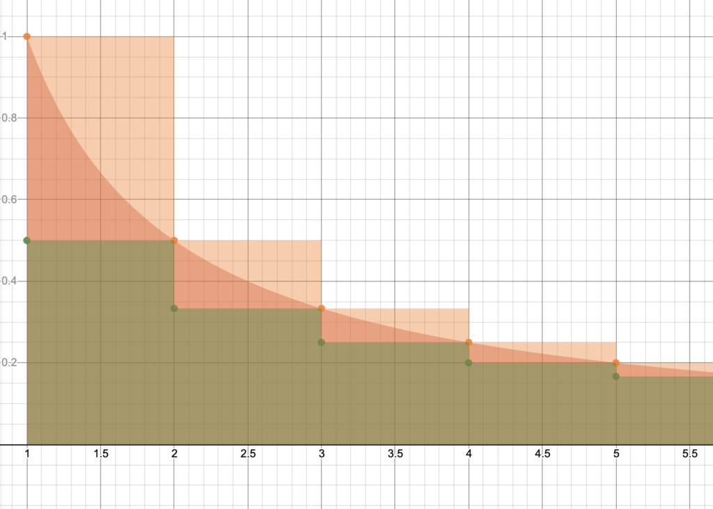
To visualize this, consider the following plot where the orange-filled area is $\sum_{k = 1}^n \frac{1}{k}$ , the green-filled area is $\sum_{k = 1}^n \frac{1}{k + 1}$ , and the red-filled area is $\int_1^n \frac{1}{x}$ .

Since $\int_1^n \frac{1}{x} = \ln(x)$ , we have $H_n = \Theta(\log n)$ . Thus we can substitue to get

$\begin{align*}\sum_{i < j} \EX[X_{i, j}] = O(n \log n)\end{align*}$

as desired. Hence, Randomized QuickSort has an expected run-time of $O(n \log n)$ . $\blacksquare$

Thus we recognize that the expected run-time of the Randomized QuickSort algorithm is quite optimal, asymptotically on par with the best sorting algorithms. In fact, sorting algorithms that only utilize comparisons all have a run-time of at least $\Omega(n \log n)$ . Furthermore, the run-time of Randomized QuickSort, in general, is concentrated around the expected run-time which we discuss in another blog. Although in practical use, this sorting algorithm has proven itself as widely efficient, it is always special to see it backed by theoretical knowledge as we have here.

Recent Posts

Recent Comments

Subscribe

Categories

Archives

Analysis of Randomized QuickSort

Expected Run-time vs. Average Run-time

Empirical Motivation

Brute-Force Analysis

Preliminaries of a Simpler Analysis

The Probabilistic Analysis

About the Author

Balaram Behera

Leave a Reply Cancel reply

You may also like these

Randomized QuickSort

Reservoir Sampling: Uniform Sampling of Streaming Data